2  Cómo funciona el aprendizaje supervisado

Veremos el caso de las máquinas de soporte vectorial (SVM) para clasificación.

• Paso #1: Cargar librerías

import matplotlib.pyplot as plt

from sklearn import svm
from sklearn.datasets import make_blobs
from sklearn.inspection import DecisionBoundaryDisplay

from scipy.stats import distributions
from numpy import sum
import numpy as np

• Paso #2: Crear datos

Se crean 40 puntos usando la función make_blobs. Esta crea un conjunto de puntos separados en dos grupos.

X, y = make_blobs(n_samples=40, centers=2, random_state=6)

• Paso #3: Crear el modelo

clf = svm.SVC(kernel="linear", C=1000)

• Paso #4: Entrenar el modelo

clf.fit(X, y)

SVC(C=1000, kernel='linear')

In a Jupyter environment, please rerun this cell to show the HTML representation or trust the notebook.
On GitHub, the HTML representation is unable to render, please try loading this page with nbviewer.org.

• Paso #5: Visualizar el modelo

plt.scatter(X[:, 0], X[:, 1], c=y, s=30, cmap=plt.cm.Paired)

# plot the decision function
ax = plt.gca()
DecisionBoundaryDisplay.from_estimator(
    clf,
    X,
    plot_method="contour",
    colors="k",
    levels=[-1, 0, 1],
    alpha=0.5,
    linestyles=["--", "-", "--"],
    ax=ax,
)
# plot support vectors
ax.scatter(
    clf.support_vectors_[:, 0],
    clf.support_vectors_[:, 1],
    s=100,
    linewidth=1,
    facecolors="none",
    edgecolors="k",
)
plt.show()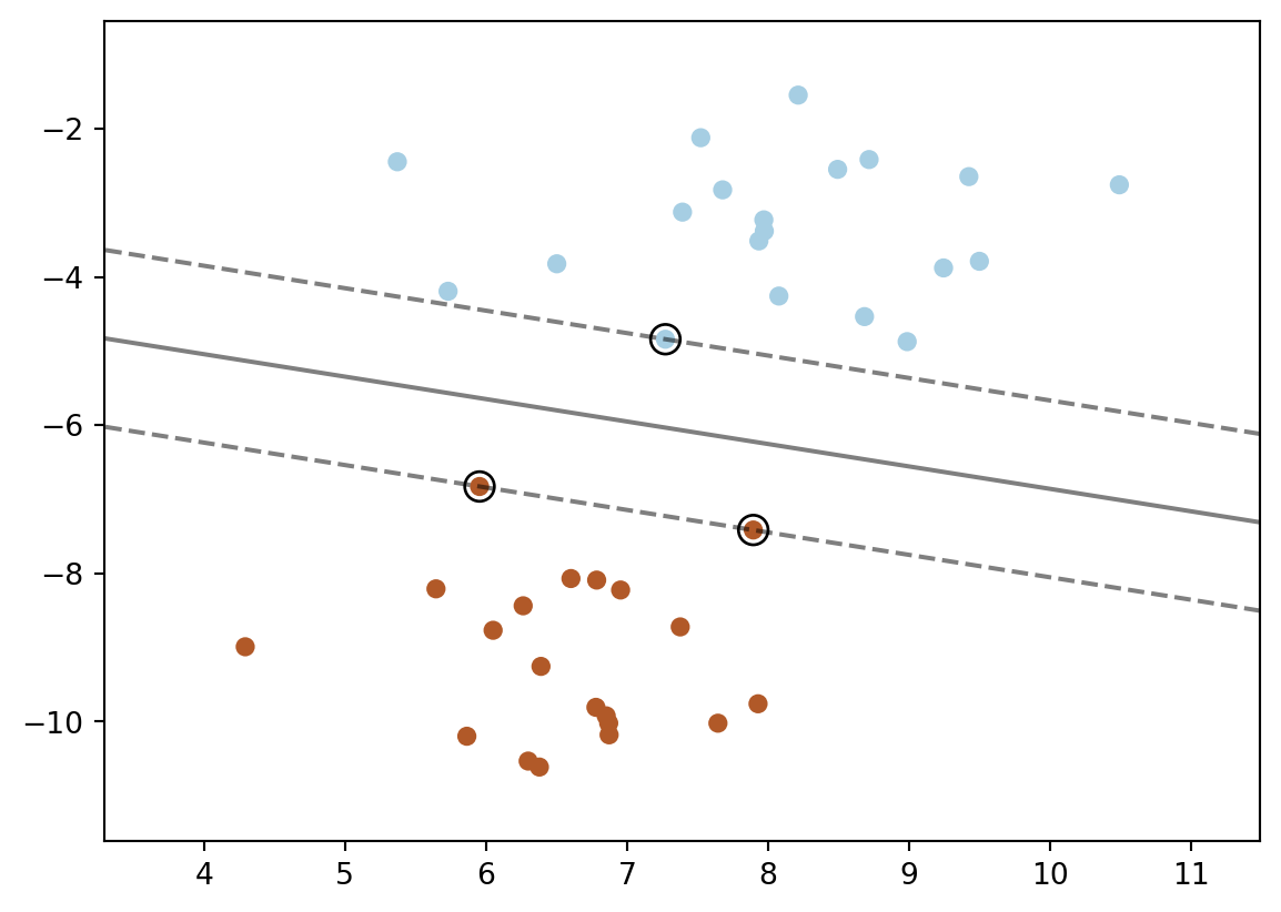

• Referencias

  1. https://scikit-learn.org/stable/modules/svm.html#
  2. https://scikit-learn.org/stable/auto_examples/svm/plot_separating_hyperplane.html#sphx-glr-auto-examples-svm-plot-separating-hyperplane-py

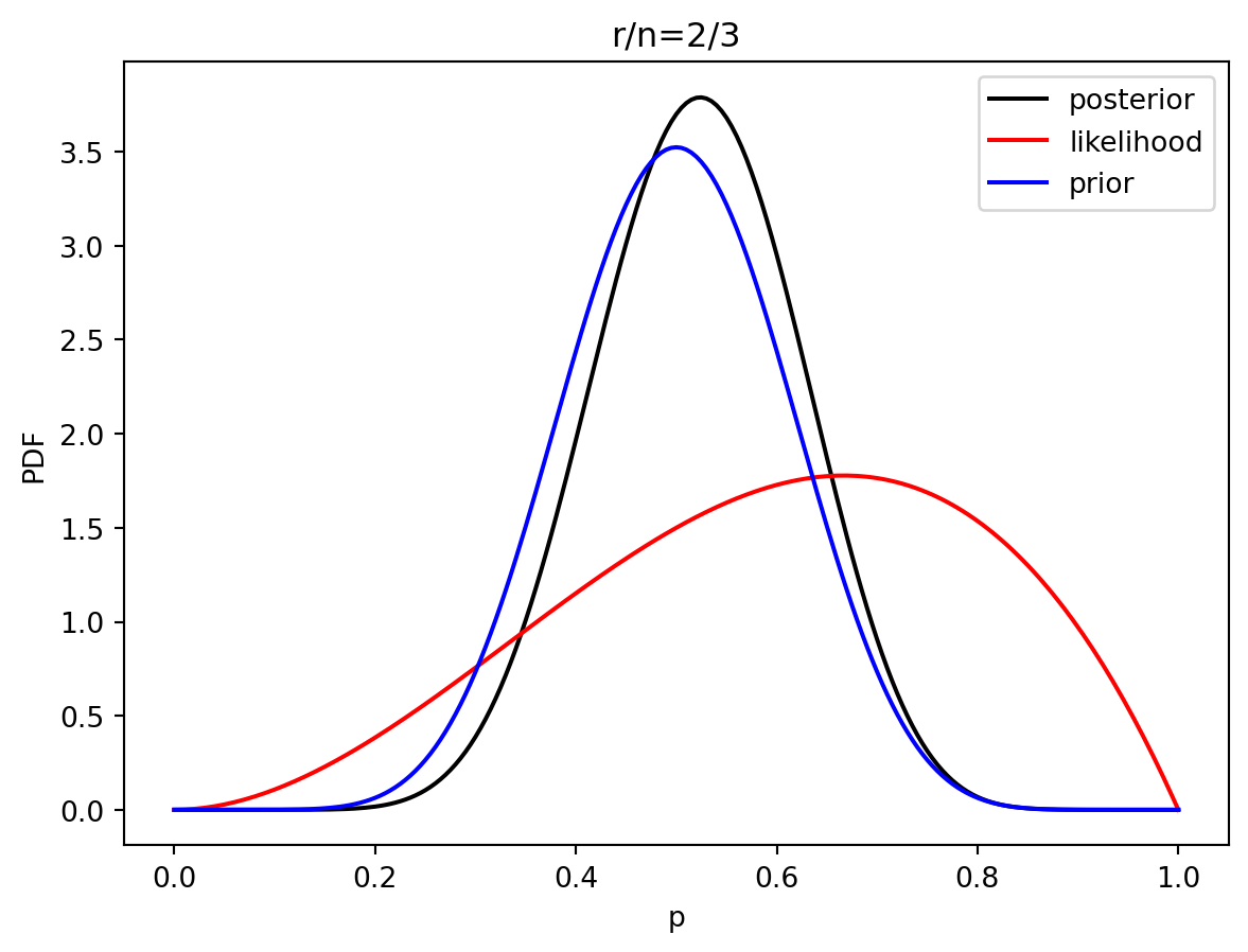
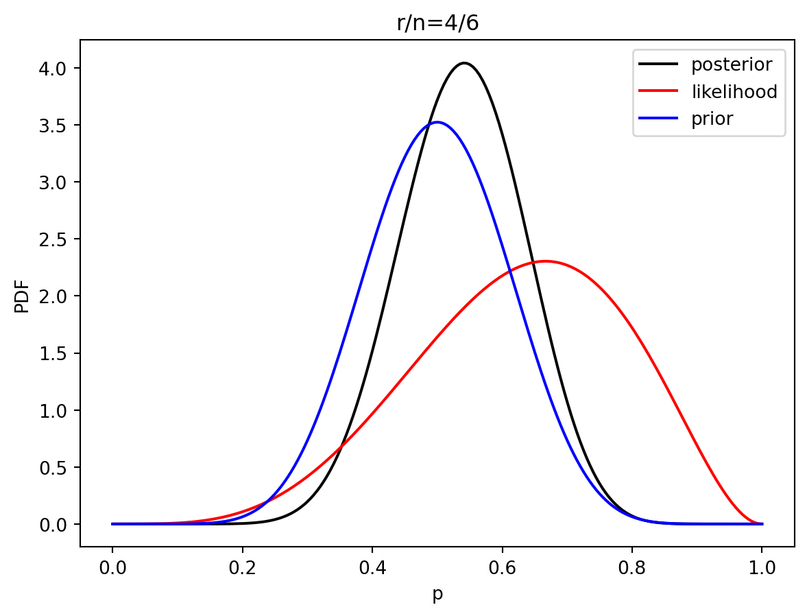
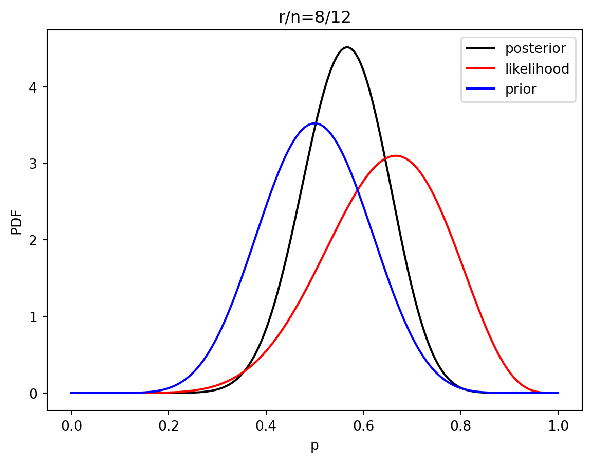
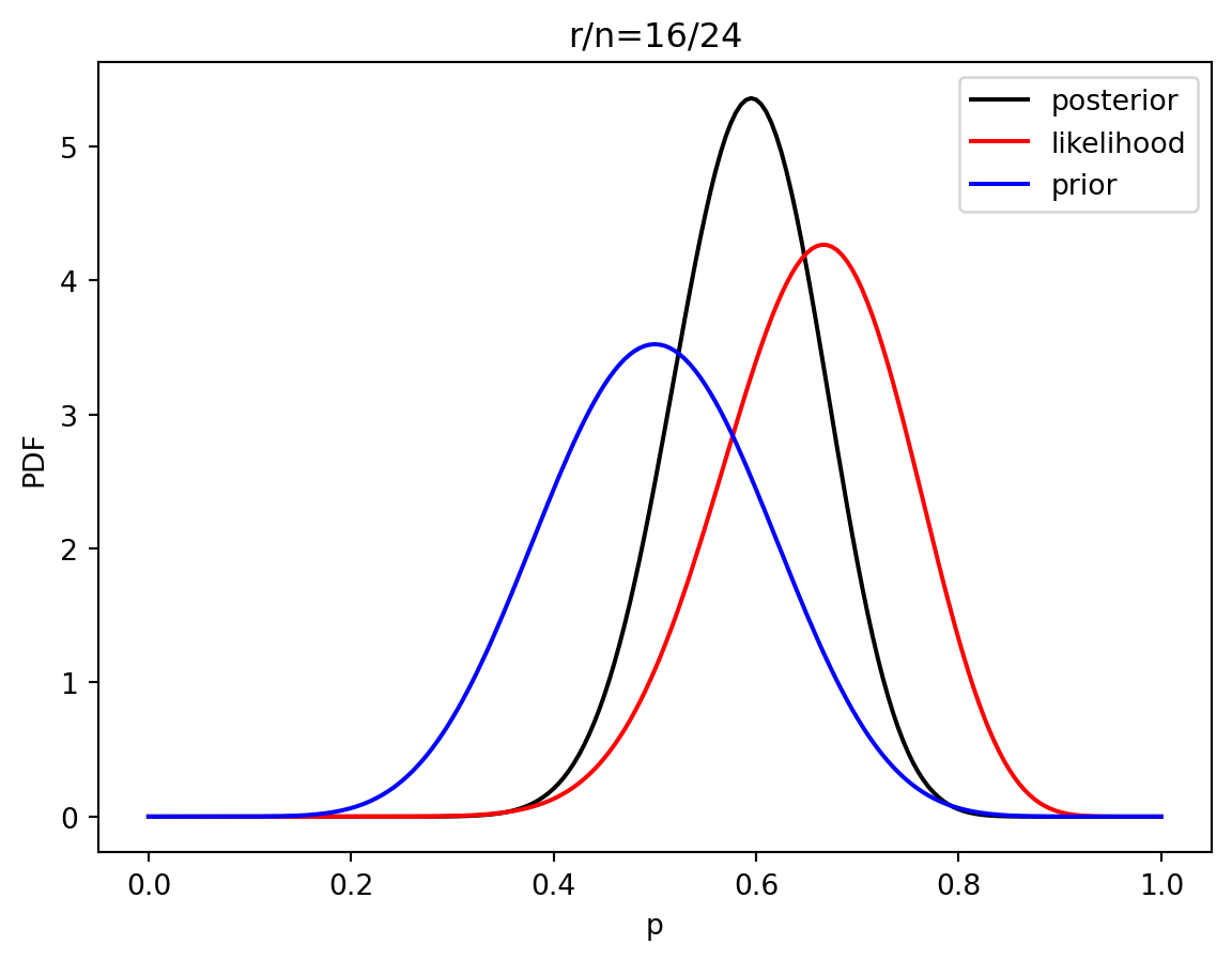
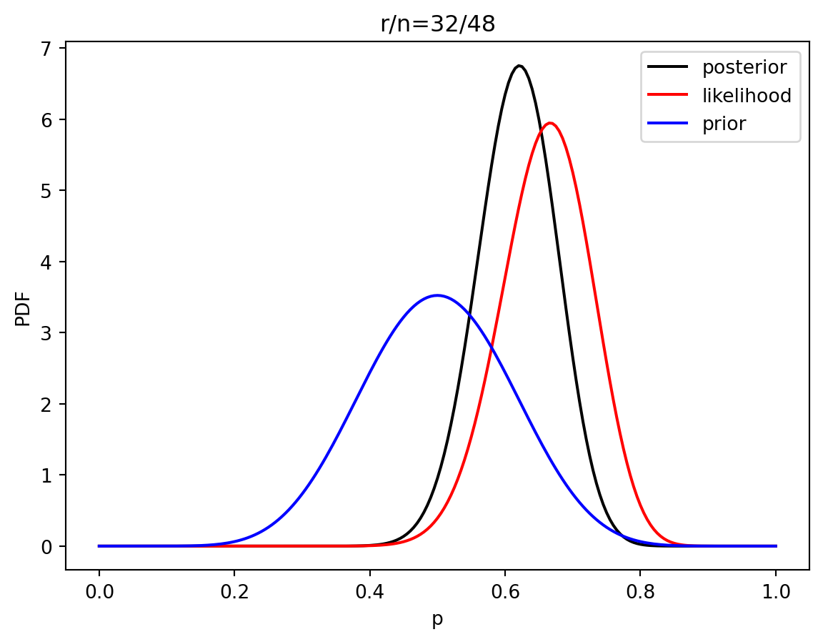
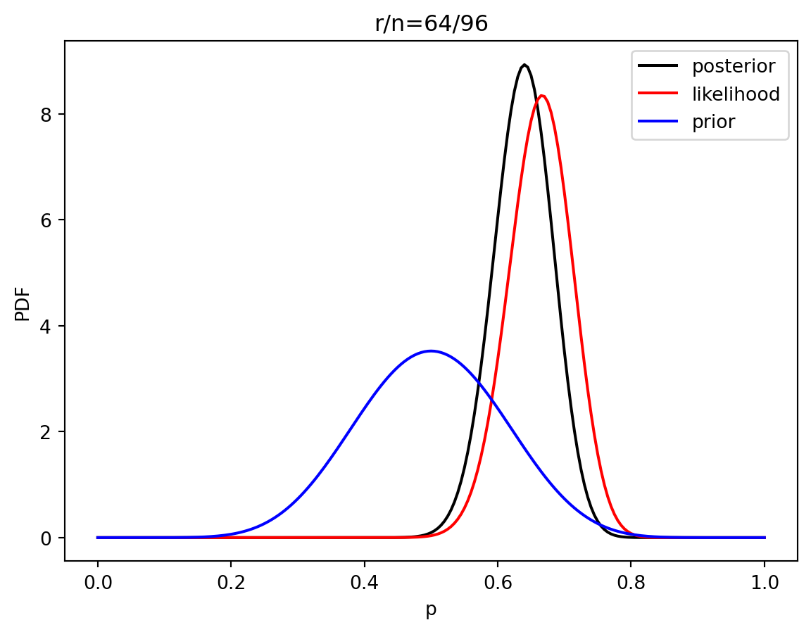
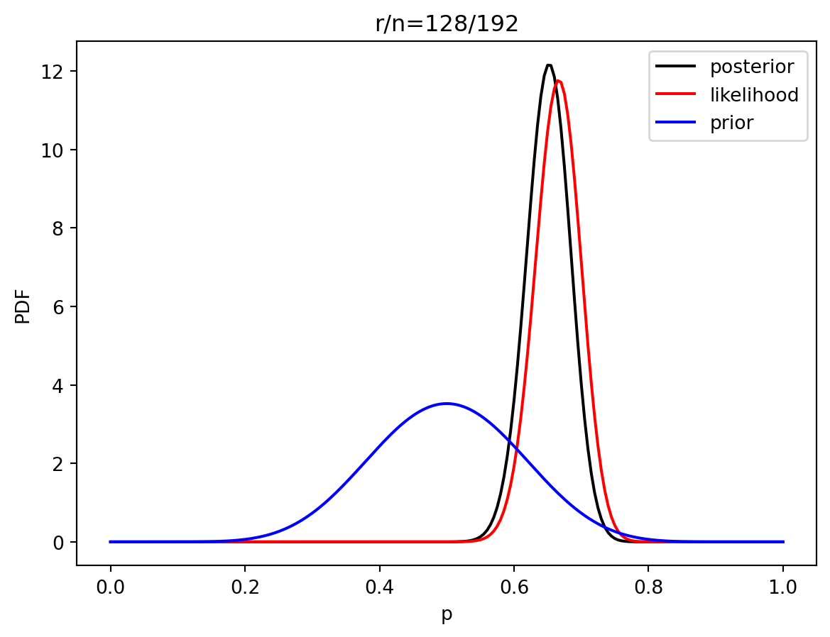
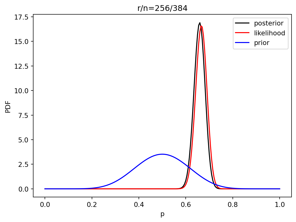
3 Estimación de parametros bayesiano

alpha = 10
beta = 10
n = 20
Nsamp = 201  # no of points to sample at
p = np.linspace(0, 1, Nsamp)
deltap = 1./(Nsamp-1)  # step size between samples of p

prior = distributions.beta.pdf(p, alpha, beta)

for i in range(1, 9):

    r = 2**i
    n = (3.0/2.0)*r
    like = distributions.binom.pmf(r, n, p)
    like = like/(deltap*sum(like))  # for plotting convenience only
    post = distributions.beta.pdf(p, alpha+r, beta+n-r)

    # make the figure
    plt.figure()
    plt.plot(p, post, 'k', label='posterior')
    plt.plot(p, like, 'r', label='likelihood')
    plt.plot(p, prior, 'b', label='prior')
    plt.xlabel('p')
    plt.ylabel('PDF')
    plt.legend(loc='best')
    plt.title('r/n={}/{:.0f}'.format(r, n))
    plt.show()